For tabular data -- spreadsheets, databases, structured business data -- tree-based methods routinely outperform neural networks. This surprises people who associate "state-of-the-art AI" with deep learning. But Kaggle competitions on tabular data are dominated by XGBoost and LightGBM, not neural networks. Understanding why requires understanding what decision trees do, how random forests fix their weaknesses, and where gradient boosting pushes performance further.
Decision Trees and Random Forests Explained: When Tree Methods Beat Neural Networks
Decision trees overfit easily. Random forests fix this by averaging many trees. XGBoost pushes further with gradient boosting. Here is when tree methods beat neural networks.

Mahmudul Haque Qudrati
CEO & ML Engineer
May 18, 2026
10 min read
One AI engineering post, weekly
LLM benchmarks, prompt techniques, and token-cost breakdowns — not another AI news roundup.
A decision tree is a flowchart. At each node, the tree asks a yes/no question about a feature: "Is the user's age greater than 35?" "Is the transaction amount more than $500?" "Is the account less than 30 days old?"
Based on the answer, data flows left or right down the tree. This continues until a leaf node, which outputs a prediction: a class label for classification, a numeric value for regression.
Training a decision tree means finding the best set of questions. "Best" is defined by an impurity measure. For classification, the most common is Gini impurity (how often a randomly chosen element would be incorrectly labeled if randomly labeled according to the distribution in the node). For regression, it is variance.
At each node, the algorithm searches over all features and all possible split thresholds to find the split that maximally reduces impurity. This search is greedy -- it finds the locally optimal split at each step rather than globally optimizing the entire tree.
The result is an interpretable model. You can follow the path from root to leaf for any prediction and explain exactly why the model made that decision. This interpretability has real business value in regulated industries (credit scoring, medical diagnosis, legal decisions) where "the model said so" is not an acceptable explanation.
The Fundamental Problem: Overfitting
Decision trees overfit aggressively if left unconstrained. A fully grown tree will create one leaf per training example, achieving perfect training accuracy and zero generalization ability. The tree has memorized rather than learned.
The standard remedy is pruning: limit tree depth, require a minimum number of samples at each leaf, or stop splitting when the improvement falls below a threshold. This reduces overfitting but creates a new problem: a single pruned tree has high variance. Change the training data slightly and you get a substantially different tree.
This variance problem motivates ensemble methods.
Team workspace
Ship faster with chat, meetings, and projects in one place — Zlyqor.
Random Forests: Ensemble Averaging
Random forests build many decision trees and average their predictions. The key insight: if individual trees have high variance but low bias, averaging many uncorrelated trees dramatically reduces variance while preserving the low bias.
Two mechanisms ensure the trees are sufficiently uncorrelated:
Bootstrap sampling (bagging). Each tree is trained on a different random sample of the training data, drawn with replacement. About 37% of the original data is excluded from each tree's training set. This means each tree sees a somewhat different dataset.
Feature subsampling. At each split, the tree is only allowed to consider a random subset of features (typically the square root of the total number of features for classification, or one third for regression). This forces trees to use different features, further decorrelating them.
The result: 100 or 500 trees, each somewhat wrong in a different way. Their errors cancel when averaged. The ensemble prediction is far more stable than any individual tree.
Random forests also provide a bonus: out-of-bag (OOB) error estimation. Because each tree was not trained on approximately 37% of the data, you can use those excluded examples to estimate generalization error without a separate validation set.
Feature importance falls out naturally: features that appear in more splits, higher in the trees, and reduce impurity more are more important. This is an interpretability advantage over neural networks.
XGBoost and Gradient Boosting
Random forests build trees in parallel (each tree is independent). Gradient boosting builds trees sequentially. Each tree is trained specifically to correct the errors of the ensemble so far.
The first tree predicts the target directly. The second tree predicts the residuals (errors) of the first tree. The third tree predicts the residuals of the first two trees combined. And so on. The final prediction is the sum of all trees' outputs.
"Gradient" in gradient boosting refers to using the gradient of the loss function to determine what each tree should predict. This is conceptually similar to gradient descent, but instead of updating continuous weights, you are adding new trees.
XGBoost (eXtreme Gradient Boosting) made gradient boosting practical at scale by adding: regularization terms (L1 and L2) directly in the objective function to control tree complexity, an efficient split-finding algorithm that handles missing values natively, column and row subsampling similar to random forests, and hardware-aware parallelism for fast training.
LightGBM from Microsoft and CatBoost from Yandex are alternative implementations with additional innovations (histogram-based splitting, native categorical feature handling). In practice, XGBoost, LightGBM, and CatBoost are all competitive and the differences matter less than hyperparameter tuning.
When Tree Methods Beat Neural Networks
Neural networks dominate images, audio, and text. For tabular data, the picture is different.
Small to medium datasets. Neural networks require large amounts of data to realize their capacity advantage. On datasets with thousands to hundreds of thousands of rows, tree methods with proper hyperparameter tuning typically match or beat neural networks with far less effort.
Heterogeneous features. Tabular data often mixes numeric features on very different scales (age in years, income in dollars, number of clicks) with categorical features (country, product category, user tier). Tree methods handle this naturally. Neural networks require careful preprocessing.
Missing values. XGBoost handles missing values natively by learning which branch to take when a feature is missing. Neural networks require explicit imputation strategies.
Interpretability requirements. A single shallow decision tree is fully explainable to a non-technical stakeholder. Even random forests provide meaningful feature importance scores. When a business or regulator needs to understand why a decision was made, tree methods are far easier to explain.
Training speed and compute constraints. Training an XGBoost model on a million-row dataset takes minutes on a laptop. Training a competitive neural network on the same data could take hours on a GPU.
When Neural Networks Win
Neural networks win when: you have very large datasets (tens of millions of rows or more), the relationships between features are highly non-linear and require deep composition, you can invest in feature engineering specifically designed for the architecture, or the data is not truly tabular (e.g., text encoded as counts, image features flattened, time series).
For a concrete benchmark: on most Kaggle tabular competitions with fewer than 10 million rows, XGBoost or LightGBM with careful tuning will be in the top solutions. Neural networks occasionally win when ensemble with tree methods, or when the data has strong sequential or spatial structure that tree methods cannot capture.
Practical Starting Point
For any new tabular ML problem:
- Start with a random forest with default hyperparameters. This gives you a strong baseline in 10 minutes.
- Switch to XGBoost or LightGBM and tune learning rate, max depth, number of trees, and regularization.
- Only consider neural networks if the tree models plateau well below your performance target or if the data has structure (sequences, spatial patterns) that trees cannot exploit.
Tree methods are not inferior to neural networks. They are the right tool for a different domain, and knowing when to use each is a fundamental ML engineering skill.
Keep Reading
- Feature Engineering Practical Guide -- tree methods benefit enormously from good features, and feature importance from trees guides where to invest
- ML Model Evaluation Metrics Guide -- how to correctly measure whether your tree model is actually better
- Machine Learning Complete Guide for Software Developers -- where tree methods fit in the full ML landscape
Pristren builds AI-powered software for teams. Zlyqor is our all-in-one workspace -- chat, projects, time tracking, AI meeting summaries, and invoicing -- in one tool. Try it free.
#decision-trees#random-forests#xgboost#gradient-boosting#tabular-data
Mahmudul Haque Qudrati
CEO & ML Engineer
Visionary technologist, software engineer, and machine learning specialist. Founder and CEO of Pristren, directing engineering teams that ship production-grade AI/ML pipelines, mission-critical full-stack applications, and developer tooling. Creator of Zlyqor, the unified team workspace platform. Author of 540+ technical guides and benchmark research reports on large language models, agentic workflows, Model Context Protocol (MCP), and modern web stacks.

More from Mahmudul
Machine Learning: Complete Guide for Software Developers
11 min read
GPT-6 Astra AGI: How to Actually Use It and Get Its Best Performance
8 min read
DeepSeek vs MiniMax vs Kimi in Coding Benchmarks: Real Scores, Real Prices, Real Tradeoffs
8 min read
GPT-6 Astra Benchmarks, Pricing, and Safety: What Developers Need to Know
5 min read
Related Articles
 11 min read
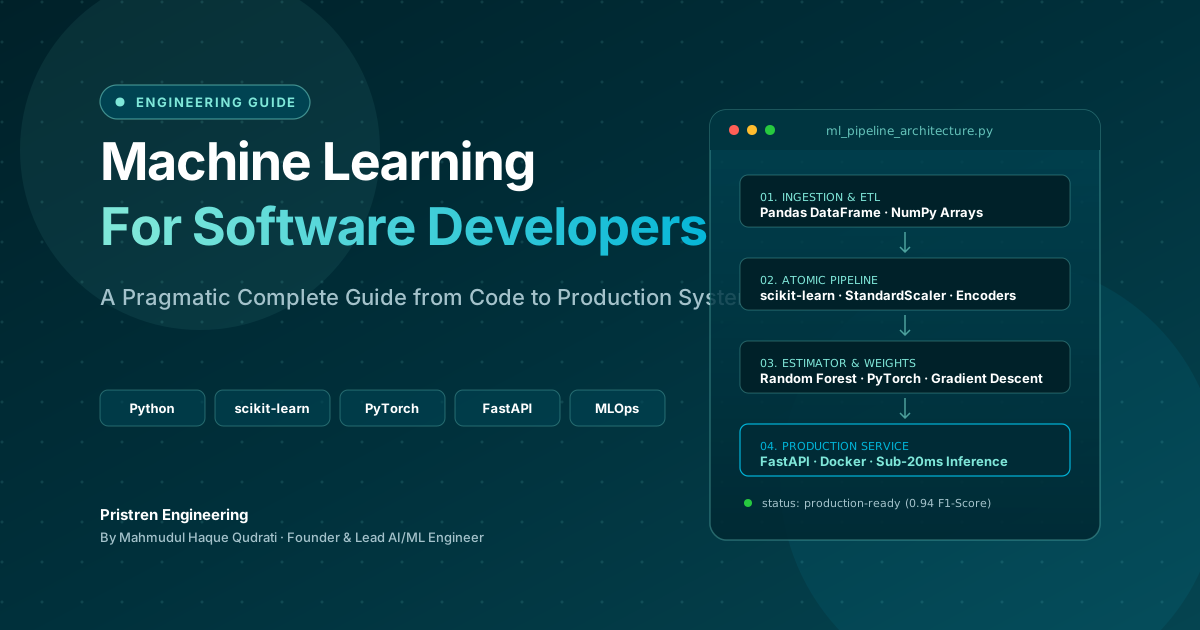
Machine Learning: Complete Guide for Software Developers
Learn machine learning as a software developer with this complete guide covering Python, algorithms, mathematics, projects, deep learning, and a practical roadmap.
 7 min read
ONNX: Export Any ML Model and Run It Anywhere
ONNX (Open Neural Network Exchange) is the universal model format - export from PyTorch, scikit-learn, or HuggingFace and run 3x faster inference with ONNX Runtime on CPU or GPU.
 10 min read
Supervised Learning Explained: How Models Learn from Labeled Examples
Supervised learning is the most widely used ML paradigm. Here is exactly how the train-measure-adjust loop works, where labels come from, and when the approach breaks down.
// discussion
Comments